FPGA開発日記

カテゴリ別記事インデックス https://msyksphinz.github.io/github_pages , English Version https://fpgadevdiary.hatenadiary.com/

RocketChipの足回りを理解する(1. RocketChipのVerilogを読み解く)

RISC-VのUCB実装であるRocketChipはRISC-Vのプロセッサ実装の中で最も参考になるもので、例えばSoCに組み込むとなると真っ先に導入を考えるRISC-V IPの一つだ。

RocketChipはデフォルトで64ビット命令をサポートしており、シンプルなパイプラインながら性能もソコソコ出る、と言うことを謳っている(まあそれが真実かは分からないけれども)。

RocketChipのコアだけを取り出して他のSoCに組み込みたいとき、または自分のバスにRocketChipを接続したいときに、どのようにすればよいのだろう? 適当にgithubから取得してきた環境でMakeして、とりあえずVerilatorでシミュレーションして終わるのならば可能だが、実際のインプリメンテーションとなるとRocketChipは分からないことが多い。 特に足回りの部分だ。

今回は、RocketChipの足回りの構成について、Scalaの実装部分と、出力されたVerilogの部分を見ながら比較、調査してみる。

RockeChipのサンプルデザインで構築される環境

今回は、VerilatorのVCDも分かりにくい、家にVCSなんてライセンスの必要なシミュレータなんて持っているはずもない、という環境のため、QuestaSim Starter Editionを使ってシミュレーションをする環境を構築した。

RocketChipのリポジトリをcloneしてくると、シミュレーション用のディレクトリとして、

  • emulator : Verilatorを使ったシミュレーション
  • vsim : VCSを使ったシミュレーション

ディレクトリが作成されるらしい。何故Questaが無いのだ!という話はあるかもしれないが、これはDPIの仕様などが微妙に異なるためと予想する。

ただし今回はDPIなんて使わずに基本的にリセット解除して、フェッチして、デコードして実行ができればよいので、無駄なものはいろいろ切り取ってシンプルな構成に変更していく。

この結果、RocketChipのデザインで生成されるRTLシミュレーション環境は、大まかに言って以下のような関係になっている。

  • TestDriver
  • TestHarness
  • ExampleRocketTop
  • 足回りの部品など
  • SRAMなど
  • coreplex

このCoreplexというものが実際のRocketCoreだと予想するが、確証はない。そこから先も大量のモジュールがインスタンスされているので、正直どこがコア部分なのか良く分からないのだ。

このcoreplexというモジュールは、RocketPlex_coreplexというモジュールになっている。Verilogファイルを参照してみる。Verilogファイルはrocket-chip/emulator/generated-src/freechips.rocketchip.chipDefaultcConfig.vに格納されている。

module RocketPlex_coreplex(
  input         clock,
  input         reset,
  input         io_interrupts_0_0,
  input         io_interrupts_0_1,
  output        io_l2in_0_a_ready,
  input         io_l2in_0_a_valid,
  input  [2:0]  io_l2in_0_a_bits_opcode,
  input  [2:0]  io_l2in_0_a_bits_param,
  input  [3:0]  io_l2in_0_a_bits_size,
  input  [3:0]  io_l2in_0_a_bits_source,
  input  [31:0] io_l2in_0_a_bits_address,
  input  [7:0]  io_l2in_0_a_bits_mask,
...

大きく分けて以下のバスが搭載されている。

  • io_l2in : External –> coreplex (L2関係?)
  • io_mmio : coreplex –> External (IOMMU関係?)
  • io_mem : coreplex –> External (命令、データフェッチ関係?)
  • io_debug : External –> coreplex (デバッグ関係?)

f:id:msyksphinz:20170712013910p:plain

良く分からないのだけれど、これらのバスはTileLinkと呼ばれるものだろうか?生成されたVerilogの中にも、TLBufferなどというモジュールでは、

module TLBuffer_fsb(
  output        io_in_0_a_ready,
  input         io_in_0_a_valid,
  input  [2:0]  io_in_0_a_bits_opcode,
  input  [2:0]  io_in_0_a_bits_param,
  input  [3:0]  io_in_0_a_bits_size,
  input  [3:0]  io_in_0_a_bits_source,
  input  [31:0] io_in_0_a_bits_address,
  input  [7:0]  io_in_0_a_bits_mask,
  input  [63:0] io_in_0_a_bits_data,
...

という感じでこのバスプロトコルが使われている。これも含め要調査だな。

CNTK 2.0 のチュートリアル試行: CNTK 103 Recognize hand written digits (OCR) with MNIST data

CNTK 2.0のチュートリアルを試行する。

今回はある程度翻訳という形で実施してみた。だいぶ誤訳はあるだろうが、ザックリ概要をつかむという形でやっていきたい。

CNTK 103のチュートリアルは4編で構成されている。MNISTの数値認識のチュートリアルについて、

  • 103 Part-A : MNIST data preparation
  • 103 Part-B : Multi-class logistic regression classifier
  • 103 Part-C : Multi-layer perception classifier
  • 103 Part-D : Convolutional neural network classifier

となっている。ここでは、すべての章を詳細にみていくと大変なので、ザックリと1つの項目にまとめた。 最初の準備段階のところとかはかなり被っているので省略している。 それぞれ、MNISTの問題を

  • ロジスティック回帰分析を用いて実現する
  • パーセプション分類器(MLP)を用いて実現する
  • 畳み込みニューラルネットワークを使って実現する

と3種類の方法をCNTKで実装し比較検討を行っている。

github.com

以降の文章については、CNTK 2.0の翻訳を含んでいるが、誤訳を含んでいる可能性がある。勉強しながら書き進めていった翻訳兼メモのため、文章の構成にはあまり力を注いでいない。

問題がある場合は指摘していただけるとありがたいです。


from IPython.display import display, Image

CNTK 103 Part A: MNIST Data Loader

CNTKでのMNISTを実施する。CNTK 101とCNTK 102のようなデータではなく、実際のデータを使用して実施していく。

  • Part A: MNISTデータベースについてまずは慣れる。
  • 後続のPart: MNISTを使用して異なるネットワークを構成する。
# 後々使用する関連モジュールをインポートする
from __future__ import print_function
import gzip
import matplotlib.image as mpimg
import matplotlib.pyplot as plt
import numpy as np
import os
import shutil
import struct
import sys
import time

try: 
    from urllib.request import urlretrieve 
except ImportError: 
    from urllib import urlretrieve

# matplotlibをインラインで利用できるようにする
%matplotlib inline

データダウンロード

MNISTデータベースはマシンラーニングアルゴリズムにおいて非常に一般的に使用されている手書きデータである。 トレーニングには60000個のデータを使用しており、10000個のデータをテストに利用している。各データには28x28ピクセルのデータで構成されている。 このデータセットはトレーニングのデータを可視化しやすいものである。

# Functions to load MNIST images and unpack into train and test set.
# - loadData reads image data and formats into a 28x28 long array
# - loadLabels reads the corresponding labels data, 1 for each image
# - load packs the downloaded image and labels data into a combined format to be read later by 
#   CNTK text reader 

def loadData(src, cimg):
    print ('Downloading ' + src)
    gzfname, h = urlretrieve(src, './delete.me')
    print ('Done.')
    try:
        with gzip.open(gzfname) as gz:
            n = struct.unpack('I', gz.read(4))
            # Read magic number.
            if n[0] != 0x3080000:
                raise Exception('Invalid file: unexpected magic number.')
            # Read number of entries.
            n = struct.unpack('>I', gz.read(4))[0]
            if n != cimg:
                raise Exception('Invalid file: expected {0} entries.'.format(cimg))
            crow = struct.unpack('>I', gz.read(4))[0]
            ccol = struct.unpack('>I', gz.read(4))[0]
            if crow != 28 or ccol != 28:
                raise Exception('Invalid file: expected 28 rows/cols per image.')
            # Read data.
            res = np.fromstring(gz.read(cimg * crow * ccol), dtype = np.uint8)
    finally:
        os.remove(gzfname)
    return res.reshape((cimg, crow * ccol))

def loadLabels(src, cimg):
    print ('Downloading ' + src)
    gzfname, h = urlretrieve(src, './delete.me')
    print ('Done.')
    try:
        with gzip.open(gzfname) as gz:
            n = struct.unpack('I', gz.read(4))
            # Read magic number.
            if n[0] != 0x1080000:
                raise Exception('Invalid file: unexpected magic number.')
            # Read number of entries.
            n = struct.unpack('>I', gz.read(4))
            if n[0] != cimg:
                raise Exception('Invalid file: expected {0} rows.'.format(cimg))
            # Read labels.
            res = np.fromstring(gz.read(cimg), dtype = np.uint8)
    finally:
        os.remove(gzfname)
    return res.reshape((cimg, 1))

def try_download(dataSrc, labelsSrc, cimg):
    data = loadData(dataSrc, cimg)
    labels = loadLabels(labelsSrc, cimg)
    return np.hstack((data, labels))

データのダウンロード

MNISTデータはトレーニングデータとテストデータから構成されている。 60000個のイメージデータと10000個のテストデータから構成されている。 まずはこのデータをダウンロードする。

# URLs for the train image and labels data
url_train_image = 'http://yann.lecun.com/exdb/mnist/train-images-idx3-ubyte.gz'
url_train_labels = 'http://yann.lecun.com/exdb/mnist/train-labels-idx1-ubyte.gz'
num_train_samples = 60000

print("Downloading train data")
train = try_download(url_train_image, url_train_labels, num_train_samples)


url_test_image = 'http://yann.lecun.com/exdb/mnist/t10k-images-idx3-ubyte.gz'
url_test_labels = 'http://yann.lecun.com/exdb/mnist/t10k-labels-idx1-ubyte.gz'
num_test_samples = 10000

print("Downloading test data")
test = try_download(url_test_image, url_test_labels, num_test_samples)
Downloading train data
Downloading http://yann.lecun.com/exdb/mnist/train-images-idx3-ubyte.gz
Done.
Downloading http://yann.lecun.com/exdb/mnist/train-labels-idx1-ubyte.gz
Done.
Downloading test data
Downloading http://yann.lecun.com/exdb/mnist/t10k-images-idx3-ubyte.gz
Done.
Downloading http://yann.lecun.com/exdb/mnist/t10k-labels-idx1-ubyte.gz
Done.

データの可視化

# Plot a random image
sample_number = 5001
plt.imshow(train[sample_number,:-1].reshape(28,28), cmap="gray_r")
plt.axis('off')
print("Image Label: ", train[sample_number,-1])

f:id:msyksphinz:20170709223811p:plain

イメージの保存

MNISTのデータは、ベクトルにフラットに保存されている(28x28のイメージデータは、784個のデータポイントに変換されて保存されている)。

ラベルはワンホットデータに変換されている(10個の分類データで、3は0001000000として表現されている)

# Save the data files into a format compatible with CNTK text reader
def savetxt(filename, ndarray):
    dir = os.path.dirname(filename)

    if not os.path.exists(dir):
        os.makedirs(dir)

    if not os.path.isfile(filename):
        print("Saving", filename )
        with open(filename, 'w') as f:
            labels = list(map(' '.join, np.eye(10, dtype=np.uint).astype(str)))
            for row in ndarray:
                row_str = row.astype(str)
                label_str = labels[row[-1]]
                feature_str = ' '.join(row_str[:-1])
                f.write('|labels {} |features {}\n'.format(label_str, feature_str))
    else:
        print("File already exists", filename)
# Save the train and test files (prefer our default path for the data)
data_dir = os.path.join("..", "Examples", "Image", "DataSets", "MNIST")
if not os.path.exists(data_dir):
    data_dir = os.path.join("data", "MNIST")

print ('Writing train text file...')
savetxt(os.path.join(data_dir, "Train-28x28_cntk_text.txt"), train)

print ('Writing test text file...')
savetxt(os.path.join(data_dir, "Test-28x28_cntk_text.txt"), test)

print('Done')
Writing train text file...
File already exists data\MNIST\Train-28x28_cntk_text.txt
Writing test text file...
File already exists data\MNIST\Test-28x28_cntk_text.txt
Done
from IPython.display import Image

CNTK 103: Part-B - 回帰分析

CNTK 103: Part-C - マルチレイヤパーセプションによるMNIST

CNTK 103: Part-D - 畳み込みニューラルネットワークによるMNIST

まずはMNISTに必要なデータを用意ししている。手書きの文字を認識する。

# Figure 1
Image(url= "http://3.bp.blogspot.com/_UpN7DfJA0j4/TJtUBWPk0SI/AAAAAAAAABY/oWPMtmqJn3k/s1600/mnist_originals.png", width=200, height=200)

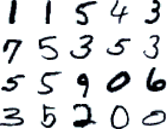
目的 MNISTのデータセットを使って、数字の認識分類器のトレーニングを実施する。

アプローチ チュートリアルで説明した同じような手順を踏む。データ読み込み、データ処理、モデルの生成、モデルパラメータの学習、モデルの評価である。

  • データ読み込み: CNTKのテキストリーダを使用する。
  • データのプリプロセッシング: Part-Aで紹介済み。

ロジスティック回帰

ロジスティック回帰(LR)は基本的な機械学習の手法であり、線形の重み分析を行い、各クラスについて確率に基づく予測を行う。

ロジスティック回帰には2種類が存在し、Binary LRは2つのクラスを予測する場合でも1つの出力を生成し、Multinomial LRは複数のクラスを予測する場合では複数の出力を生成する。

Image(url="https://camo.githubusercontent.com/2eb7e133489dbf4eb253c271b2688056be84dbe0/687474703a2f2f7777772e636e746b2e61692f6a75702f636e746b313033625f54776f466f726d734f664c522d76332e706e67")

# 関連するコンポーネントをロードする
from __future__ import print_function # Use a function definition from future version (say 3.x from 2.7 interpreter)
import matplotlib.image as mpimg
import matplotlib.pyplot as plt
import numpy as np
import sys
import os

import cntk as C

%matplotlib inline
# Select the right target device when this notebook is being tested:
if 'TEST_DEVICE' in os.environ:
    if os.environ['TEST_DEVICE'] == 'cpu':
        C.device.try_set_default_device(C.device.cpu())
    else:
        C.device.try_set_default_device(C.device.gpu(0))

初期化

# 常に同じ乱数が生成できるように調整
np.random.seed(0)

# データ次元を定義する
input_dim = 784
num_output_classes = 10

データ読み込み

MNISTのデータは60000個のトレーニングセットを持っており、10000個のテストセットを持っている。

# テキストフォーマットのCTFを読み込む(ファイルからのCFTデシリアライザを読み込む)
def create_reader(path, is_training, input_dim, num_label_classes):
    
    labelStream = C.io.StreamDef(field='labels', shape=num_label_classes, is_sparse=False)
    featureStream = C.io.StreamDef(field='features', shape=input_dim, is_sparse=False)
    
    deserailizer = C.io.CTFDeserializer(path, C.io.StreamDefs(labels = labelStream, features = featureStream))
            
    return C.io.MinibatchSource(deserailizer,
       randomize = is_training, max_sweeps = C.io.INFINITELY_REPEAT if is_training else 1)
# トレーニングデータとテストデータの生成
# それぞれ配列を定義し格納する。
data_found = False

for data_dir in [os.path.join("..", "Examples", "Image", "DataSets", "MNIST"),
                 os.path.join("data", "MNIST")]:
    train_file = os.path.join(data_dir, "Train-28x28_cntk_text.txt")
    test_file = os.path.join(data_dir, "Test-28x28_cntk_text.txt")
    if os.path.isfile(train_file) and os.path.isfile(test_file):
        data_found = True
        break
        
if not data_found:
    raise ValueError("Please generate the data by completing CNTK 103 Part A")
    
print("Data directory is {0}".format(data_dir))
Data directory is data\MNIST

ロジスティック回帰のモデル生成

ロジスティック回帰(logistic regression: LR)ネットワークは機械学習の世界において過去10年で使われてきた、シンプルなビルディングブロックを使用した効率的なネットワークである。

Image(url="https://camo.githubusercontent.com/0fc29e9645a061453403af37d46750beb2d91356/68747470733a2f2f7777772e636e746b2e61692f6a75702f636e746b313033625f4d4e4953545f4c522e706e67")

input = C.input_variable(input_dim)
label = C.input_variable(num_output_classes)

def create_model(features):
    with C.layers.default_options(init = C.glorot_uniform()):
        r = C.layers.Dense(num_output_classes, activation = None)(features)
        return r

# Scale the input to 0-1 range by dividing each pixel by 255.
z = create_model(input/255.0)
# Define a utility function to compute the moving average sum.
# A more efficient implementation is possible with np.cumsum() function
def moving_average(a, w=5):
    if len(a) < w:
        return a[:]    # Need to send a copy of the array
    return [val if idx < w else sum(a[(idx-w):idx])/w for idx, val in enumerate(a)]


# Defines a utility that prints the training progress
def print_training_progress(trainer, mb, frequency, verbose=1):
    training_loss = "NA"
    eval_error = "NA"

    if mb%frequency == 0:
        training_loss = trainer.previous_minibatch_loss_average
        eval_error = trainer.previous_minibatch_evaluation_average
        if verbose: 
            print ("Minibatch: {0}, Loss: {1:.4f}, Error: {2:.2f}%".format(mb, training_loss, eval_error*100))
        
    return mb, training_loss, eval_error
# ネットワークの初期化を行う
minibatch_size = 64
num_samples_per_sweep = 60000
num_sweeps_to_train_with = 10
num_minibatches_to_train = (num_samples_per_sweep * num_sweeps_to_train_with) / minibatch_size

loss = C.cross_entropy_with_softmax(z, label)
label_error = C.classification_error(z, label)

# モデルトレーニングを駆動させるためのトレーナをインスタンスする
learning_rate = 0.2
lr_schedule = C.learning_rate_schedule(learning_rate, C.UnitType.minibatch)
learner = C.sgd(z.parameters, lr_schedule)
trainer = C.Trainer(z, (loss, label_error), [learner])

# トレーニングデータセットを生成する
reader_train = create_reader(train_file, True, input_dim, num_output_classes)

# データストリームを入力とラベルにマップする
input_map = {
    label  : reader_train.streams.labels,
    input  : reader_train.streams.features
} 

# トレーニングを実行する
training_progress_output_freq = 500

plotdata = {"batchsize":[], "loss":[], "error":[]}

for i in range(0, int(num_minibatches_to_train)):
    
    # トレーニングデータファイルにミニバッチを適用する
    data = reader_train.next_minibatch(minibatch_size, input_map = input_map)
    
    trainer.train_minibatch(data)
    batchsize, loss, error = print_training_progress(trainer, i, training_progress_output_freq, verbose=1)
    
    if not (loss == "NA" or error =="NA"):
        plotdata["batchsize"].append(batchsize)
        plotdata["loss"].append(loss)
        plotdata["error"].append(error)
Minibatch: 0, Loss: 2.2132, Error: 79.69%
Minibatch: 500, Loss: 0.5081, Error: 12.50%
Minibatch: 1000, Loss: 0.2309, Error: 4.69%
Minibatch: 1500, Loss: 0.4300, Error: 15.62%
Minibatch: 2000, Loss: 0.1918, Error: 6.25%
Minibatch: 2500, Loss: 0.1843, Error: 7.81%
Minibatch: 3000, Loss: 0.1117, Error: 1.56%
Minibatch: 3500, Loss: 0.3094, Error: 12.50%
Minibatch: 4000, Loss: 0.3554, Error: 10.94%
Minibatch: 4500, Loss: 0.2465, Error: 4.69%
Minibatch: 5000, Loss: 0.1988, Error: 3.12%
Minibatch: 5500, Loss: 0.1277, Error: 4.69%
Minibatch: 6000, Loss: 0.1448, Error: 3.12%
Minibatch: 6500, Loss: 0.2789, Error: 9.38%
Minibatch: 7000, Loss: 0.1692, Error: 6.25%
Minibatch: 7500, Loss: 0.3069, Error: 9.38%
Minibatch: 8000, Loss: 0.1194, Error: 3.12%
Minibatch: 8500, Loss: 0.1464, Error: 4.69%
Minibatch: 9000, Loss: 0.1096, Error: 3.12%
# Compute the moving average loss to smooth out the noise in SGD
plotdata["avgloss"] = moving_average(plotdata["loss"])
plotdata["avgerror"] = moving_average(plotdata["error"])

# Plot the training loss and the training error
import matplotlib.pyplot as plt

plt.figure(1)
plt.subplot(211)
plt.plot(plotdata["batchsize"], plotdata["avgloss"], 'b--')
plt.xlabel('Minibatch number')
plt.ylabel('Loss')
plt.title('Minibatch run vs. Training loss')

plt.show()

plt.subplot(212)
plt.plot(plotdata["batchsize"], plotdata["avgerror"], 'r--')
plt.xlabel('Minibatch number')
plt.ylabel('Label Prediction Error')
plt.title('Minibatch run vs. Label Prediction Error')
plt.show()

f:id:msyksphinz:20170709223851p:plain

f:id:msyksphinz:20170709223857p:plain

ロジスティック回帰の評価 / テスト

トレーニングの完了したネットワークで、テストを実施する。

# トレーニングデータを読み込む
reader_test = create_reader(test_file, False, input_dim, num_output_classes)

test_input_map = {
    label  : reader_test.streams.labels,
    input  : reader_test.streams.features,
}

# テストデータを読み込む
test_minibatch_size = 512
num_samples = 10000
num_minibatches_to_test = num_samples // test_minibatch_size
test_result = 0.0

for i in range(num_minibatches_to_test):
    
    # test_minibatch_size のバッチサイズでテストデータをロードする。
    # 784ピクセルのMNISTデータをロードする
    data = reader_test.next_minibatch(test_minibatch_size,
                                      input_map = test_input_map)

    eval_error = trainer.test_minibatch(data)
    test_result = test_result + eval_error

# 全てのミニバッチテストに対して平均エラー率を計算する
print("Average test error: {0:.2f}%".format(test_result*100 / num_minibatches_to_test))
Average test error: 7.41%

マルチレイヤパーセプションのモデル生成

マルチレイヤパーセプションは2レイヤの隠しレイヤ(num_hidden_layers)の、比較的シンプルなネットワークである。

Image(url="https://camo.githubusercontent.com/173a509c6aab581dc9f2e872f56a349883b1776d/687474703a2f2f636e746b2e61692f6a75702f636e746b313033635f4d4e4953545f4d4c502e706e67")

num_hidden_layers = 2
hidden_layers_dim = 400

input = C.input_variable(input_dim)
label = C.input_variable(num_output_classes)

def create_model(features):
    with C.layers.default_options(init = C.layers.glorot_uniform(), activation = C.ops.relu):
            h = features
            for _ in range(num_hidden_layers):
                h = C.layers.Dense(hidden_layers_dim)(h)
            r = C.layers.Dense(num_output_classes, activation = None)(h)
            return r
        
z = create_model(input)

# Scale the input to 0-1 range by dividing each pixel by 255.
z = create_model(input/255.0)
loss = C.cross_entropy_with_softmax(z, label)
label_error = C.classification_error(z, label)

# Instantiate the trainer object to drive the model training
learning_rate = 0.2
lr_schedule = C.learning_rate_schedule(learning_rate, C.UnitType.minibatch)
learner = C.sgd(z.parameters, lr_schedule)
trainer = C.Trainer(z, (loss, label_error), [learner])

# Initialize the parameters for the trainer
minibatch_size = 64
num_samples_per_sweep = 60000
num_sweeps_to_train_with = 10
num_minibatches_to_train = (num_samples_per_sweep * num_sweeps_to_train_with) / minibatch_size

# Create the reader to training data set
reader_train = create_reader(train_file, True, input_dim, num_output_classes)

# Map the data streams to the input and labels.
input_map = {
    label  : reader_train.streams.labels,
    input  : reader_train.streams.features
} 

# Run the trainer on and perform model training
training_progress_output_freq = 500

plotdata = {"batchsize":[], "loss":[], "error":[]}

for i in range(0, int(num_minibatches_to_train)):
    
    # Read a mini batch from the training data file
    data = reader_train.next_minibatch(minibatch_size, input_map = input_map)
    
    trainer.train_minibatch(data)
    batchsize, loss, error = print_training_progress(trainer, i, training_progress_output_freq, verbose=1)
    
    if not (loss == "NA" or error =="NA"):
        plotdata["batchsize"].append(batchsize)
        plotdata["loss"].append(loss)
        plotdata["error"].append(error)
Minibatch: 0, Loss: 2.3329, Error: 95.31%
Minibatch: 500, Loss: 0.2762, Error: 7.81%
Minibatch: 1000, Loss: 0.0661, Error: 1.56%
Minibatch: 1500, Loss: 0.1294, Error: 6.25%
Minibatch: 2000, Loss: nan, Error: 92.19%
Minibatch: 2500, Loss: nan, Error: 93.75%
Minibatch: 3000, Loss: nan, Error: 90.62%
Minibatch: 3500, Loss: nan, Error: 85.94%
Minibatch: 4000, Loss: nan, Error: 92.19%
Minibatch: 4500, Loss: nan, Error: 90.62%
Minibatch: 5000, Loss: nan, Error: 95.31%
Minibatch: 5500, Loss: nan, Error: 84.38%
Minibatch: 6000, Loss: nan, Error: 87.50%
Minibatch: 6500, Loss: nan, Error: 87.50%
Minibatch: 7000, Loss: nan, Error: 82.81%
Minibatch: 7500, Loss: nan, Error: 95.31%
Minibatch: 8000, Loss: nan, Error: 89.06%
Minibatch: 8500, Loss: nan, Error: 96.88%
Minibatch: 9000, Loss: nan, Error: 92.19%
# Compute the moving average loss to smooth out the noise in SGD
plotdata["avgloss"] = moving_average(plotdata["loss"])
plotdata["avgerror"] = moving_average(plotdata["error"])

# Plot the training loss and the training error
import matplotlib.pyplot as plt

plt.figure(1)
plt.subplot(211)
plt.plot(plotdata["batchsize"], plotdata["avgloss"], 'b--')
plt.xlabel('Minibatch number')
plt.ylabel('Loss')
plt.title('Minibatch run vs. Training loss')

plt.show()

plt.subplot(212)
plt.plot(plotdata["batchsize"], plotdata["avgerror"], 'r--')
plt.xlabel('Minibatch number')
plt.ylabel('Label Prediction Error')
plt.title('Minibatch run vs. Label Prediction Error')
plt.show()

f:id:msyksphinz:20170709223912p:plain

f:id:msyksphinz:20170709223915p:plain

マルチレイヤパーセプションの評価/テスト

# トレーニングデータの読み込み
reader_test = create_reader(test_file, False, input_dim, num_output_classes)

test_input_map = {
    label  : reader_test.streams.labels,
    input  : reader_test.streams.features,
}

# トレーニングのモデル読み込み
test_minibatch_size = 512
num_samples = 10000
num_minibatches_to_test = num_samples // test_minibatch_size
test_result = 0.0

for i in range(num_minibatches_to_test):
    
    # We are loading test data in batches specified by test_minibatch_size
    # Each data point in the minibatch is a MNIST digit image of 784 dimensions 
    # with one pixel per dimension that we will encode / decode with the 
    # trained model.
    data = reader_test.next_minibatch(test_minibatch_size,
                                      input_map = test_input_map)

    eval_error = trainer.test_minibatch(data)
    test_result = test_result + eval_error

# Average of evaluation errors of all test minibatches
print("Average test error: {0:.2f}%".format(test_result*100 / num_minibatches_to_test))
Average test error: 90.20%

畳み込みニューラルネットワークのモデル生成

入力次元

畳み込みニューラルネットワークの入力データは3Dマトリックス(チャネル,画像の幅,画像の高さ)にて構成される

# 乱数をシードを固定して再現性を持たせる
np.random.seed(0)

# データの次元を定義する
input_dim_model = (1, 28, 28)    # 28 x 28 with 1 チャネルの画像を定義する
input_dim = 28*28                # 画像データをベクトルとして定義する
num_output_classes = 10

CNNは複数のレイヤから構成されるネットワークであり、あるレイヤの出力が次のレイヤの入力になるようなネットワークである。 これはマルチレイヤパーセプション(Multi Layer Perception: MLP)と似ている。 MLPはすべてのピクセルの入力ペアを出力をすべて接続されている。したがって、組み合わせ爆発が発生するのと、オーバフィッティングが発生しやすい。 畳み込みレイヤは、ピクセルの空間は位置関係を活用して、ネットワーク中のパラメータの数を減らすことができる。 フィルタのサイズは畳み込みレイヤのパラメータである。

畳み込みレイヤ

畳み込みレイヤはフィルタの集合である。各フィルタは重み \bf W と バイアス bから構成される。 これらのフィルタは画像内をスキャンし、画像とのドットプロダクトを計算し、バイアスを加算する。ドットプロダクトの値を活性化関数に渡す。

Image(url="https://www.cntk.ai/jup/cntk103d_conv2d_final.gif", width= 300)

畳み込みレイヤには以下の特徴がある。

  • 入力と出力が完全接続されたレイヤと異なり、畳み込みノードは入力ノードの一部とその隣接するローカルノードでのみ接続される。これはreceptive field(RF)と呼ばれる。上図では3x3の領域がRF領域である。RGBの場合には、画像は3つの3×3の領域があり、3つの色チャネルのそれぞれが1つ存在する。

  • Denseレイヤのような単一の重みレイヤの代わりに、畳み込みレイヤは複数の重みの集合を持っている(上図ではそれぞれ別の色で表現されている)。これをフィルタと呼ぶ。各フィルタは入力画像の受信フィールドの特徴を検出する。畳み込みの出力はサブレイヤの一部である(下記のアニメーションに示す)。ここでnはフィルタの数である。

  • サブレイヤの中では、各ノードが自分自身の重み情報を持つ代わりに、サブレイヤ中では同じ重み情報が利用される。これによりパラメータの数を減らし、学習のオーバフィッティングを防いでいる。この軽量化により、ディープラーニングのさまざな実際の問題で問題を解決可能にしている:

  • より大きな画像の処理 (512 x 512など)
  • より大きなフィルタサイズを使用する (11 x 11など)
  • より多くのフィルタを学習させる(128など)
  • よりレイヤ数の深いアーキテクチャを実現する(100+のレイヤなど)
  • 変換の不変性を達成する(画像内のどの領域にあっても認識することができるような能力)

Strides and Pad parameters

ストライドとPadパラメータ

フィルタをどのように配置するのか? 一般的に、フィルタはおーばラップしたタイルのように配置され、左から右方向へ、上から下へと進んでいく。 各畳み込みレイヤはfilter_shapeを指定するパラメータを持っており、ほとんど自然な画像の場合にフィルタの幅と高さを指定するパラメータを持っている。また、フィルタが画像内を移動する場合にどの程度のステップで移動するかを指定するためのパラメータ(stride)が存在する。 booleanのパラメータであるpadは入力値が境界線の近くでのタイルどりを可能にするために、入力がパディングされるかどうかを制御する。

上記のアニメーションではfilter_shape = (3, 3), strides = (2, 2), pad = Falseの場合の処理を表現している。 次のアニメーションでは、padTrueに設定している。 最初のアニメーションではstrideは2だが、次のアニメーションではstrideは1である。 ここで、出力値の形(最も下のレイヤ)はそれぞれのストライドの設定により異なっている。 padおよびstrideの値の決定は、出力レイヤの必要な形により決定される。

# Plot images with strides of 2 and 1 with padding turned on
images = [("https://www.cntk.ai/jup/cntk103d_padding_strides.gif" , 'With stride = 2'),
          ("https://www.cntk.ai/jup/cntk103d_same_padding_no_strides.gif", 'With stride = 1')]

for im in images:
    print(im[1])
    display(Image(url=im[0], width=200, height=200))
With stride = 2

With stride = 1

CNNモデルの構築

本CNNのチュートリアルでは、最初に2つのコンテナを定義する。 1つ目のコンテナはMNIST画像を入力するためのもので、2つ目のものは10個の数字へのラベリングを行うためのものである。 データを読み込んだ時、readerは自動的に1画像あたり784ピクセルinput_dim_modelのタプルへと変換する (この例では (1, 28, 28)

x = C.input_variable(input_dim_model)
y = C.input_variable(num_output_classes)

最初のモデルは、単純な畳み込みのみのモデルである。 ここでは2つの畳み込みモデルを持っており、MNISTの10個の数値を検出することが目的であるから、幅10のベクトルがネットワークの出力であり、各ベクトルの要素が各数字に相当する。 これは、num_output_classのdenseレイヤの出力を使って、最後の畳み込み層の出力を反映することで可能となる。 このチュートリアルの前に、ロジスティック回帰およびMLPでは最後のレイヤでクラスの数分だけマッピングされることを見た。 また、トレーニング中にcross entropy損失関数を使用したsoftmax関数を利用することにより、最後のdenseレイヤは活性化関数を持っていない。

以下の図は我々が構築しようとしているネットワークのモデルである。 このモデル内のパラメータは実験に使用されることに注意すること。 これらはネットワークのハイパーパラメータと呼ばれる。 フィルタの形が増大すると、モデルパラメータの数も増え、計算時間も増大し、モデルがデータにフィットすることを助ける。 しかし、オーバフィッティングのリスクもある。 典型的に、より深い層のレイヤのフィルタの数はそれより前のレイヤのフィルタよりも大きい。 私たちは最初のレイヤで8、次のレイヤで16のフィルタを選択した。 これらのハイパーパラメータはモデル構築中に実験されるべきである。

Image(url="https://camo.githubusercontent.com/a157ed88853727d46ecbdc11fa0dcc868804c247/68747470733a2f2f7777772e636e746b2e61692f6a75702f636e746b313033645f636f6e766f6e6c79322e706e67")

x = C.input_variable(input_dim_model)
y = C.input_variable(num_output_classes)

# function to モデルの構築

def create_model(features):
    with C.layers.default_options(init=C.glorot_uniform(), activation=C.relu):
            h = features
            h = C.layers.Convolution2D(filter_shape=(5,5), 
                                       num_filters=8, 
                                       strides=(2,2), 
                                       pad=True, name='first_conv')(h)
            h = C.layers.Convolution2D(filter_shape=(5,5), 
                                       num_filters=16, 
                                       strides=(2,2), 
                                       pad=True, name='second_conv')(h)
            r = C.layers.Dense(num_output_classes, activation=None, name='classify')(h)
            return r
        
# モデルのインスタンス
z = create_model(x)

# ネットワークの出力形式をプリントする。
print("Output Shape of the first convolution layer:", z.first_conv.shape)
print("Bias value of the last dense layer:", z.classify.b.value)

# ネットワーク中のパラメータ
C.logging.log_number_of_parameters(z)
Output Shape of the first convolution layer: (8, 14, 14)
Bias value of the last dense layer: [ 0.  0.  0.  0.  0.  0.  0.  0.  0.  0.]
Training 11274 parameters in 6 parameter tensors.

モデルパラメータの学習

前回のチュートリアルと同様に、softmax関数を使用してevidenceもしくは活性化された値を確率に変換する。

トレーニング

CNTK 102と同様に、cross-entropyを最小化することを目的とする。 最終的な値が想定と異なるならば、CNTK 102を再度見てほしい。 複数のモデルを効率的にビルドするために、いくつかのサポート関数を用意している。

def create_criterion_function(model, labels):
    loss = C.cross_entropy_with_softmax(model, labels)
    errs = C.classification_error(model, labels)
    return loss, errs # (model, labels) -> (loss, error metric)

def train_test(train_reader, test_reader, model_func, num_sweeps_to_train_with=10):
    
    # Instantiate the model function; x is the input (feature) variable 
    # We will scale the input image pixels within 0-1 range by dividing all input value by 255.
    model = model_func(x/255)
    
    # Instantiate the loss and error function
    loss, label_error = create_criterion_function(model, y)
    
    # Instantiate the trainer object to drive the model training
    learning_rate = 0.2
    lr_schedule = C.learning_rate_schedule(learning_rate, C.UnitType.minibatch)
    learner = C.sgd(z.parameters, lr_schedule)
    trainer = C.Trainer(z, (loss, label_error), [learner])
    
    # Initialize the parameters for the trainer
    minibatch_size = 64
    num_samples_per_sweep = 60000
    num_minibatches_to_train = (num_samples_per_sweep * num_sweeps_to_train_with) / minibatch_size
    
    # Map the data streams to the input and labels.
    input_map={
        y  : train_reader.streams.labels,
        x  : train_reader.streams.features
    } 
    
    # Uncomment below for more detailed logging
    training_progress_output_freq = 500
     
    # Start a timer
    start = time.time()

    for i in range(0, int(num_minibatches_to_train)):
        # Read a mini batch from the training data file
        data=train_reader.next_minibatch(minibatch_size, input_map=input_map) 
        trainer.train_minibatch(data)
        print_training_progress(trainer, i, training_progress_output_freq, verbose=1)
     
    # Print training time
    print("Training took {:.1f} sec".format(time.time() - start))
    
    # Test the model
    test_input_map = {
        y  : test_reader.streams.labels,
        x  : test_reader.streams.features
    }

    # Test data for trained model
    test_minibatch_size = 512
    num_samples = 10000
    num_minibatches_to_test = num_samples // test_minibatch_size

    test_result = 0.0   

    for i in range(num_minibatches_to_test):
    
        # We are loading test data in batches specified by test_minibatch_size
        # Each data point in the minibatch is a MNIST digit image of 784 dimensions 
        # with one pixel per dimension that we will encode / decode with the 
        # trained model.
        data = test_reader.next_minibatch(test_minibatch_size, input_map=test_input_map)
        eval_error = trainer.test_minibatch(data)
        test_result = test_result + eval_error

    # Average of evaluation errors of all test minibatches
    print("Average test error: {0:.2f}%".format(test_result*100 / num_minibatches_to_test))

トレーニングの実行とテストの実施

これで、畳み込みニューラルネットワークの構築が完了した。

def do_train_test():
    global z
    z = create_model(x)
    reader_train = create_reader(train_file, True, input_dim, num_output_classes)
    reader_test = create_reader(test_file, False, input_dim, num_output_classes)
    train_test(reader_train, reader_test, z)
    
do_train_test()
Minibatch: 0, Loss: 2.3157, Error: 96.88%
Minibatch: 500, Loss: 0.1691, Error: 9.38%
Minibatch: 1000, Loss: 0.0890, Error: 1.56%
Minibatch: 1500, Loss: 0.1083, Error: 3.12%
Minibatch: 2000, Loss: 0.0115, Error: 0.00%
Minibatch: 2500, Loss: 0.0058, Error: 0.00%
Minibatch: 3000, Loss: 0.0049, Error: 0.00%
Minibatch: 3500, Loss: 0.0750, Error: 3.12%
Minibatch: 4000, Loss: 0.0220, Error: 0.00%
Minibatch: 4500, Loss: 0.0192, Error: 1.56%
Minibatch: 5000, Loss: 0.0101, Error: 0.00%
Minibatch: 5500, Loss: 0.0014, Error: 0.00%
Minibatch: 6000, Loss: 0.0048, Error: 0.00%
Minibatch: 6500, Loss: 0.0098, Error: 0.00%
Minibatch: 7000, Loss: 0.0079, Error: 0.00%
Minibatch: 7500, Loss: 0.0038, Error: 0.00%
Minibatch: 8000, Loss: 0.0139, Error: 0.00%
Minibatch: 8500, Loss: 0.0058, Error: 0.00%
Minibatch: 9000, Loss: 0.0148, Error: 0.00%
Training took 17.5 sec
Average test error: 1.50%
print("Bias value of the last dense layer:", z.classify.b.value)
Bias value of the last dense layer: [-0.02818329 -0.08973262  0.02727109 -0.14188322  0.0115815  -0.09806534
  0.00059815 -0.09239398  0.39416206  0.01649885]
out = C.softmax(z)
# Read the data for evaluation
reader_eval=create_reader(test_file, False, input_dim, num_output_classes)

eval_minibatch_size = 25
eval_input_map = {x: reader_eval.streams.features, y:reader_eval.streams.labels} 

data = reader_eval.next_minibatch(eval_minibatch_size, input_map=eval_input_map)

img_label = data[y].asarray()
img_data = data[x].asarray()

# reshape img_data to: M x 1 x 28 x 28 to be compatible with model
img_data = np.reshape(img_data, (eval_minibatch_size, 1, 28, 28))

predicted_label_prob = [out.eval(img_data[i]) for i in range(len(img_data))]
# Find the index with the maximum value for both predicted as well as the ground truth
pred = [np.argmax(predicted_label_prob[i]) for i in range(len(predicted_label_prob))]
gtlabel = [np.argmax(img_label[i]) for i in range(len(img_label))]
print("Label    :", gtlabel[:25])
print("Predicted:", pred)
Label    : [7, 2, 1, 0, 4, 1, 4, 9, 5, 9, 0, 6, 9, 0, 1, 5, 9, 7, 3, 4, 9, 6, 6, 5, 4]
Predicted: [7, 2, 1, 0, 4, 1, 4, 9, 5, 9, 0, 6, 9, 0, 1, 5, 9, 7, 3, 4, 9, 6, 6, 5, 4]
# Plot a random image
sample_number = 5
plt.imshow(img_data[sample_number].reshape(28,28), cmap="gray_r")
plt.axis('off')

img_gt, img_pred = gtlabel[sample_number], pred[sample_number]
print("Image Label: ", img_pred)

f:id:msyksphinz:20170709223929p:plain

プーリングレイヤ

多くの場合に、特にディープネットワークを制御する場合にはパラメータの数を制御する必要がある。 全ての畳み込みレイヤの出力(各レイヤ、フィルタの出力に相当する)では、プーリングレイヤを配置することができる。 プーリングレイヤの典型的な特徴として、

  • 前のレイヤの次元数を削減する(ネットワークを高速化する)
  • 画像内のオブジェクトの位置ずれに対しても対応できるネットワークを構築する。例えば、もし画像の位置が中央ではなく横にずれていても、分類器が分類処理を問題なく実行できるようにする。

プーリングノードの計算は、通常のフィードフォワード処理よりも簡単である。 プーリングノードには重みも、バイアスも活性化関数も存在しない。 プーリングノードは簡単な集合関数(max, 平均など)を使用して出力を計算する。 最も共通して使用されるのはmaxである。入力のフィルタ位置に対応する入力値の最大値を出力する。

以下の図は4x4の領域を持つ入力値である。 maxプーリングウィンドウサイズは2x2であり、左上のこーなから処理を開始する。 ウィンドウ内の最大値がその領域の出力値となる。 モデルは指定されたストライドパラメータでシフトしていき、maxのプーリング操作が繰り返される。

もう一つのプーリング関数は"average"である。 averageはmaxの代わりに使用される。2つのプーリング処理をそれぞれアニメーションでまとめた。

# Plot images with strides of 2 and 1 with padding turned on
images = [("https://www.cntk.ai/jup/c103d_max_pooling.gif" , 'Max pooling'),
          ("https://www.cntk.ai/jup/c103d_average_pooling.gif", 'Average pooling')]

for im in images:
    print(im[1])
    display(Image(url=im[0], width=200, height=200))
Max pooling

Average pooling

典型的な畳み込みネットワーク

典型的なCNNは複数の畳み込みレイヤとプーリングレイヤで構成されており、最後にdense出力レイヤが接続されている。 多くの分類器のディープネットワーク(VGG, AlexNetなど)のバリエーションを見つけることができるだろう。 CNTK_103Cで使用したMLPネットワークは対照的に、2つのdenseレイヤで構成されており、最後にdense出力レイヤが接続されている。

説明の図では2次元の画像処理のネットワークとして表現しているが、CNTKのコンポーネントはどのような次元のデータでも取り扱うことができる。 上位の根とワークでは2つの畳み込みレイヤと2つのmax-プーリングレイヤで構成されている。 典型的な戦略としては、より深いレイヤになるにつれてフィルタの数を増やし、中間レイヤの空間的なサイズを減らすことである。

タスク: MaxPoolingを利用したネットワークの構築

CNTKのMaxPooling関数を使用してこのタスクを実現する。create_model関数を以下のように変更して、MaxPooling操作を追加する。

# function to build model
def create_model(features):
    with C.layers.default_options(init = C.layers.glorot_uniform(), activation = C.relu):
            h = features
            
            h = C.layers.Convolution2D(filter_shape=(5,5), 
                                       num_filters=8, 
                                       strides=(1,1), 
                                       pad=True, name="first_conv")(h)
            h = C.layers.MaxPooling(filter_shape=(2,2), 
                                    strides=(2,2), name="first_max")(h)
            h = C.layers.Convolution2D(filter_shape=(5,5), 
                                       num_filters=16, 
                                       strides=(1,1), 
                                       pad=True, name="second_conv")(h)
            h = C.layers.MaxPooling(filter_shape=(3,3), 
                                    strides=(3,3), name="second_max")(h)
            r = C.layers.Dense(num_output_classes, activation = None, name="classify")(h)
            return r
        
do_train_test()
Minibatch: 0, Loss: 2.3284, Error: 95.31%
Minibatch: 500, Loss: 0.1598, Error: 7.81%
Minibatch: 1000, Loss: 0.0865, Error: 3.12%
Minibatch: 1500, Loss: 0.1355, Error: 3.12%
Minibatch: 2000, Loss: 0.0236, Error: 1.56%
Minibatch: 2500, Loss: 0.0036, Error: 0.00%
Minibatch: 3000, Loss: 0.0031, Error: 0.00%
Minibatch: 3500, Loss: 0.0744, Error: 3.12%
Minibatch: 4000, Loss: 0.0186, Error: 1.56%
Minibatch: 4500, Loss: 0.0503, Error: 1.56%
Minibatch: 5000, Loss: 0.0300, Error: 1.56%
Minibatch: 5500, Loss: 0.0176, Error: 0.00%
Minibatch: 6000, Loss: 0.0137, Error: 0.00%
Minibatch: 6500, Loss: 0.0308, Error: 1.56%
Minibatch: 7000, Loss: 0.0204, Error: 1.56%
Minibatch: 7500, Loss: 0.0040, Error: 0.00%
Minibatch: 8000, Loss: 0.0046, Error: 0.00%
Minibatch: 8500, Loss: 0.0363, Error: 3.12%
Minibatch: 9000, Loss: 0.0049, Error: 0.00%
Training took 18.4 sec
Average test error: 1.15%


CNTK 2.0 のチュートリアル試行: CNTK 102 Feed Forward network with NumPy

CNTK 2.0のチュートリアルを試行する。

今回はある程度翻訳という形で実施してみた。だいぶ誤訳はあるだろうが、ザックリ概要をつかむという形でやっていきたい。

github.com

以降の文章については、CNTK 2.0の翻訳を含んでいるが、誤訳を含んでいる可能性がある。問題がある場合は指摘していただけるとありがたいです。


from IPython.display import Image

CNTK 102: フィードフォワードネットワークを使ってデータ分類を実行する

CNTK 101では回帰分析でデータの分類を行ったが、今回はフィードフォワードネットワークを用いてデータの分類を実行する。これはCNTK 101と同じ課題を解くことになる。

問題 (CNTK 101と同様)

CNTK 101チュートリアルでは、回帰分析を用いてデータの分類を行う。ここで例として取り上げられているのは、2種類の要素(年齢、腫瘍の大きさ)に対するガン腫瘍であるかどうかを識別する回帰分析だ。つまり、X軸を年齢、Y軸を腫瘍の大きさ都市、それがガン腫瘍であるかどうかを識別するものとなる。 以下のようなグラフをプロットすることができ、青色のプロットが良性腫瘍、赤色のプロットが悪性腫瘍となる。 さらに、下記のような回帰直線を引くことで、良性と悪性の境界線を引くことができるようになる。

# Figure 1
Image(url="https://www.cntk.ai/jup/cancer_data_plot.jpg", width=400, height=400)

f:id:msyksphinz:20170708232441p:plain

CNTK 101では、回帰分析を用いてデータを分類する直線を探索した。しかし実際の世界の問題では、線形関数で分類することのできるデータというのは制度にかけ、良い特性を導くための材料としては不足だ。 個のチュートリアルでは、複数の線形関数の答えを組み合わせることによって(CNTK 101の回帰分析の回答を利用する)、非線形の分類法を導くことを目的とする。

アプローチの方法

任意の学習アルゴリズムは5つの段階を踏む。データ読み込み、データ処理、モデル作成、モデルパラメータの学習、モデルの評価(テスト、予測)である。 本チュートリアルでは、3番目のモデル作成のところのみCNTK 101と異なり、今回はフィードフォワードのネットワークを利用する。

フィードフォワードネットワークモデル

回帰モデルのチュートリアルと、同様のデータセットを使用してフィードフォワードのモデルを学習させる。このモデルでは複数の回帰分析器を利用して、単体の回帰分析よりもより複雑なデータを分類する際に適切な境界値を設定できるようにする。以下は一般的なネットワークの構成である。

# Figure 2
Image(url="https://upload.wikimedia.org/wikipedia/en/5/54/Feed_forward_neural_net.gif", width=200, height=200)

f:id:msyksphinz:20170708232511p:plain

フィードフォワードニューラルネットワークは、ネットワークのノード間で「サイクルが発生しない」ネットワークである。 フィードフォワードニューラルネットワークは人工のニューあるネットワークの中で最初に登場した、最もシンプルなネットワークである。 このネットワークでは、情報は単一の方向、順方向にのみ、入力ノードから(必要とあれば)隠しノード、そして出力ノードへと伝搬していく。 ネットワーク中にサイクルは存在しない。

チュートリアルでは、上記の5つのステップと、テストデータを用いたモデルのテストを完了させるために必要なステップとしては、異なるものを利用していく。

# Import the relevant components
from __future__ import print_function # Use a function definition from future version (say 3.x from 2.7 interpreter)
import matplotlib.pyplot as plt
%matplotlib inline

import numpy as np
import sys
import os

import cntk as C

以下のブロックでは、本チュートリアルスクリプトをCNTKで実行する場合のターゲットについて、マシン内部の定義されている環境変数を探している。 適切なターゲットデバイス(GPU vs CPU)を選択して設定する。それ以外の場合には、CNTKのデフォルトのポリ氏を利用して実行可能な最適なデバイスを利用する(使用可能ならばGPU、それ以外はCPU)

# Select the right target device when this notebook is being tested:
if 'TEST_DEVICE' in os.environ:
    if os.environ['TEST_DEVICE'] == 'cpu':
        C.device.try_set_default_device(C.device.cpu())
    else:
        C.device.try_set_default_device(C.device.gpu(0))

データの生成

本節はCNTK 101を理解しているのならばスキップすることができる。次のセクション「モデルの生成」に進んでよい。

がんのサンプルに似せた合成データを作成する。これにはPythonnumpyライブラリを利用する。ここで生成する(2次元で表現された)2つの特徴を持っており、各データは2つのクラスのうちどちらかに属している(良性データ: 青、悪性データ:赤)。

今回の例では、トレーニングデータはラベル(青もしくは赤)を持っており、各軸に対応している(ここでは2つの特性として、年齢と腫瘍の大きさを利用する)。 本例では、2つのクラスをラベル0, 1として表現する。したがって、この問題は2値の分離問題である。

# Ensure we always get the same amount of randomness
np.random.seed(0)

# Define the data dimensions
input_dim = 2
num_output_classes = 2

入力値とラベル

チュートリアルではnumpyライブラリを利用して合成データを作成する。読者が実際の世界で扱う問題では、特性データ(年齢と腫瘍の大きさ)に対して、ひとつの観察データ(observation)が存在する。 ここでは、各観察データは(もし別の特性が存在するならば)2次元のデータではなくより高次元のデータであり、それらはCNTKではテンソルとして表現される。 より高度なチュートリアルではより高い次元のデータを扱う方法についても紹介する。

# Helper function to generate a random data sample
def generate_random_data_sample(sample_size, feature_dim, num_classes):
    # Create synthetic data using NumPy. 
    Y = np.random.randint(size=(sample_size, 1), low=0, high=num_classes)

    # Make sure that the data is separable
    X = (np.random.randn(sample_size, feature_dim)+3) * (Y+1)
    X = X.astype(np.float32)    
    # converting class 0 into the vector "1 0 0", 
    # class 1 into vector "0 1 0", ...
    class_ind = [Y==class_number for class_number in range(num_classes)]
    Y = np.asarray(np.hstack(class_ind), dtype=np.float32)
    return X, Y
# Create the input variables denoting the features and the label data. Note: the input 
# does not need additional info on number of observations (Samples) since CNTK first create only 
# the network tooplogy first 
mysamplesize = 64
features, labels = generate_random_data_sample(mysamplesize, input_dim, num_output_classes)

データを可視化してみよう。

注意 mathplotlib.pyplotのインポートに失敗した場合、conda install matplotlibを実行してpyplotのバージョン依存の問題を修復すること。

# Plot the data 
import matplotlib.pyplot as plt
%matplotlib inline

# given this is a 2 class 
colors = ['r' if l == 0 else 'b' for l in labels[:,0]]

plt.scatter(features[:,0], features[:,1], c=colors)
plt.xlabel("Scaled age (in yrs)")
plt.ylabel("Tumor size (in cm)")
plt.show()

f:id:msyksphinz:20170708232658p:plain

モデルの生成

我々のフィードフォワードネットワークは比較的単純で、2つの隠れレイヤ(num_hidden_layers)を持っており、各隠れレイヤには50個の隠れノード(hidden_layer_dim)が用意されている。

# Figure 3
Image(url="http://cntk.ai/jup/feedforward_network.jpg", width=200, height=200)

f:id:msyksphinz:20170708232722p:plain

上記の緑色のノードが隠れレイヤであり、本例では50個用意されている。また隠れレイヤの数は2である。ここで次の値はどのようになるか。

  • num_hidden_layers
  • hidden_layers_dim

注意 上記の図では、(回帰分析の際に説明した)バイアスノードについては表示していない。各隠れレイヤにはバイアスノードが存在している。

num_hidden_layers = 2
hidden_layers_dim = 50

ネットワークの入力と出力は以下である。

  • 入力値(CNTKコンセプトのキーとなるもの)

入力値は、モデル観測中(つまりトレーニング中)もモデル評価中(つまりテスト中)も異なる観測データ(データポイントもしくはサンプル、本例の青赤色で表現されたもの)のコンテナである。 つまり、inputの形状は提供される出力データの形状とマッチしていなければならない。 例えば、データが縦10ピクセルx横5ピクセルのデータであれば、入力の特徴値の次元は2である(画像データの縦、横で表現される)。 同様に、本例では入力データの次元は、年齢と腫瘍サイズの2、つまりinput_dim = 2である。 別のチュートリアルでは、より多くの次元のデータの処理についても取り扱う。

問題 今回のモデルでは、入力の次元値はいくつになるか? これはCNTKのネットワークやモデルの値を理解するためには必須のものである。

# The input variable (representing 1 observation, in our example of age and size) $\bf{x}$ which 
# in this case has a dimension of 2. 
#
# The label variable has a dimensionality equal to the number of output classes in our case 2. 

input = C.input_variable(input_dim)
label = C.input_variable(num_output_classes)

フィードフォワードネットワークのセットアップ

では1ステップずつフィードフォワードネットワークを構築していこう。 最初のレイヤは次元(input_dim,  m と表記)の入力特徴ベクトル( \bf x)を入力し、いわゆるevidence((hidden_layer_dim)次元(ここでは nと表記)を受け取る隠しレイヤに向けて渡す。 入力レイヤの各特徴データは、行列 \bf W  (m \times n)で表現される重みノードに接続される。 最初のステップでは、すべての特徴データに対してevidenceを計算することである。 注意 ここでは行列、ベクトルを表現するために太字を利用している。

 \bf z_1 = W \cdot x + b

ここで bは次元 nのバイアスベクトルである。

liner_layer関数では、以下の2つの処理を行う。

  1. 特徴データ( x)と重み( W)を乗算する。
  2. バイアス項 bを加算する。
def linear_layer(input_var, output_dim):
    input_dim = input_var.shape[0]
    
    weight = C.parameter(shape=(input_dim, output_dim))
    bias = C.parameter(shape=(output_dim))

    return bias + C.times(input_var, weight)

次のステップはevidence(線形レイヤの出力)を非線形関数(いわゆる「活性化関数」)に変形することである。 活性化関数を選択して、evidenceを活性化関数に変換することになる(活性化関数は、ここから選択する)。 Sigmoid関数やTanh関数が歴史的に利用されてきている。 本チュートリアルではSigmoid関数を利用する。Sigmoid関数の出力は、しばしば次のレイヤの入力として利用され、また最終レイヤの出力として利用される。

問題 そのほかの非線形関数を使用してみよう。これらの非線形関数の使用方法について慣れてみよう。

def dense_layer(input_var, output_dim, nonlinearity):
    l = linear_layer(input_var, output_dim)
    
    return nonlinearity(l)

完全接続された分類器を作成するためには、一つ隠れレイヤを作成するとそれを次々に接続しなければならない。 最初のレイヤの出力 \bt h_1 は次のレイヤの入力となる。

本チュートリルあるのネットワークでは2層のレイヤしか使用しないので、以下のようなコードとなる。

h1 = dense_layer(input_var, hidden_layer_dim, sigmoid)
h2 = dense_layer(h1, hidden_layer_dim, sigmoid)

より多層のネットワークについて素早く評価するためには、以下のような記述でもよいだろう。

h = dense_layer(input_var, hidden_layer_dim, sigmoid)
for i in range(1, num_hidden_layers):
    h = dense_layer(h, hidden_layer_dim, sigmoid)
# Define a multilayer feedforward classification model
def fully_connected_classifier_net(input_var, num_output_classes, hidden_layer_dim, 
                                   num_hidden_layers, nonlinearity):
    
    h = dense_layer(input_var, hidden_layer_dim, nonlinearity)
    for i in range(1, num_hidden_layers):
        h = dense_layer(h, hidden_layer_dim, nonlinearity)
    
    return linear_layer(h, num_output_classes)

ネットワークの出力zはネットワーク全体の出力として使用される。

# Create the fully connected classfier
z = fully_connected_classifier_net(input, num_output_classes, hidden_layers_dim, 
                                   num_hidden_layers, C.sigmoid)

前述のネットワークの記述がCNTKのプリミティブ関数群を使用してネットワークを構築する方法を理解するのを助ける一方で、より手早く高速なネットワークを構築するためにライブラリを使用する方法もある。 CNTKは(レゴブロックのような)共通部品の「レイヤ」を用意しており、それぞれ標準的なレイヤで構成されるネットワークの設計を簡単にする。 例えば、dense_layerDenseレイヤ関数によって簡単にディープモデルとして操作できるようになっている。 入力値(Input)をモデルに渡すと、ネットワークの出力が返される。

提案されるタスク 定義されたモデルをチェックし、create_model関数の出力と下記で上記のコードをカプセル化したものを比較せよ。

def create_model(features):
    with C.layers.default_options(init=C.layers.glorot_uniform(), activation=C.sigmoid):
        h = features
        for _ in range(num_hidden_layers):
            h = C.layers.Dense(hidden_layers_dim)(h)
        last_layer = C.layers.Dense(num_output_classes, activation = None)
        
        return last_layer(h)
        
z = create_model(input)

モデルパラメータのトレーニング

ネットワークが完成したら、次にモデルパラメータ \bt W \bt bのトレーニングを行う。 まずはネットワークを通って得られた出力[tex: \bt z{final_layer}] を確率 \bt pとして変換する。 [tex: \bt p = \text{softmax}\left( \bt z\text{final_layer} \right)]

トレーニング

トレーニングを実行するためには、ネットワークを通じて得られた値と実際の答えがどれくらい異なっているかを計算する必要がある。 つまり、実際のラベルに近づくように、ネットワークを通じて得られた確率を近づけていく必要がある。 この関数は「損失関数」と呼ばれ、学習したモデルと実際のトレーニングセットの誤差を示している。

  H(p) = -\sum_{j=1}^{C} y_j\log\left( p_j \right)

 pはsoftmax関数により生成された確率であり、  yはラベルを示している。 データにより提供されたラベルは「ground-truth label」とも呼ばれる。 このチュートリアルではラベルのクラスは2だが、ラベルの値も2つのじげんを持っている(num_output_classesの値、 Cと同一である)。 一般的には、手元にあるタスクが C個の異なるクラスに分類される場合、ラベルの値は C個の要素を持ち、 Cの要素が0のところにあれば、データポイントで表されるクラスを除いて1になる。 クロスエントロピー関数については、理解することを強く推奨する。

loss = C.cross_entropy_with_softmax(z, label)

評価

分類結果を評価するためには、evidenceのベクトルとして表現されているネットワークの出力値(softmax関数により確率に変換されている)はクラスの数と同一なので、それらを比較することである。

eval_error = C.classification_error(z, label)

誤差を最小にするためには様々な手法があるが、「確率的勾配効果法(Stochastic Gradient Descent: SGD)」という手法が最も有名である。 典型的に、この方法はランダムな初期値でモデルのパラメータを設定する。 SGDの最適化器は、予測されたラベルの値とground-truthラベルとの誤差を計算し、勾配効果法を使用して次のイタレーションのモデルパラメータを生成する。

上記のモデルパラメータの更新には、メモリ中にロードされているすべてのデータセットを使用して更新するわけではないという点で魅力的である。 この手法ではより少ないデータポイントを使って重みの更新を行う。 従ってより多くのデータセットを使用してトレーニングを行うことが可能となる。 しかし、単一のサンプルによって値を更新すると、各イタレーションにて結果が大きく異なる場合がある。 ここでは、複数の小さなデータセットをロードして、誤差と損失はその平均値とし、モデルパラメータを更新する。 これをミニバッチ法と呼ぶ。

ミニバッチでは、より多くのトレーニングデータセットを使用する。 異なるトレーニングサンプルを使用してモデルパラメータの更新を繰り返し、処理時間と損失を減らしていく。 エラー率が小さくなり、大きな更新がなくなった場合に、そのモデルはトレーニングが完了したということである。

最適化の一つのカギとなるのが、learning_rateと呼ばれる値である。 この値は各イタレーションにおいて計算した値がモデルの更新にどれだけ影響を与えるのかを決める値である。 この値については、今後のチュートリアルで詳細を述べる。 これらの情報に基づいて、トレーニング器を構成していく。

# Instantiate the trainer object to drive the model training
learning_rate = 0.5
lr_schedule = C.learning_rate_schedule(learning_rate, C.UnitType.minibatch) 
learner = C.sgd(z.parameters, lr_schedule)
trainer = C.Trainer(z, (loss, eval_error), [learner])

まずは、いくつかのサポート関数を作成して、学習した結果を可視化できるようにする。

# Define a utility function to compute the moving average sum.
# A more efficient implementation is possible with np.cumsum() function
def moving_average(a, w=10):    
    if len(a) < w: 
        return a[:]    # Need to send a copy of the array
    return [val if idx < w else sum(a[(idx-w):idx])/w for idx, val in enumerate(a)]


# Defines a utility that prints the training progress
def print_training_progress(trainer, mb, frequency, verbose=1):    
    training_loss = "NA"
    eval_error = "NA"

    if mb%frequency == 0:
        training_loss = trainer.previous_minibatch_loss_average
        eval_error = trainer.previous_minibatch_evaluation_average
        if verbose: 
            print ("Minibatch: {}, Train Loss: {}, Train Error: {}".format(mb, training_loss, eval_error))
        
    return mb, training_loss, eval_error

トレーニングの実行

トレーニングを実行する。各イタレーションでは25個のサンプルを入力する。これはミニバッチのサイズと同一である。 ここでは20000個のデータを学習させる。 ちなみに実際の場合には、これと同様のラベルデータを提供する。 ここでは全体のデータセットのうち70%をトレーニングで使用し、残りはモデルの評価のために取っておくものとする。

# Initialize the parameters for the trainer
minibatch_size = 25
num_samples = 20000
num_minibatches_to_train = num_samples / minibatch_size
# Run the trainer and perform model training
training_progress_output_freq = 20

plotdata = {"batchsize":[], "loss":[], "error":[]}

for i in range(0, int(num_minibatches_to_train)):
    features, labels = generate_random_data_sample(minibatch_size, input_dim, num_output_classes)
    
    # Specify the input variables mapping in the model to actual minibatch data for training
    trainer.train_minibatch({input : features, label : labels})
    batchsize, loss, error = print_training_progress(trainer, i, 
                                                     training_progress_output_freq, verbose=0)
    
    if not (loss == "NA" or error =="NA"):
        plotdata["batchsize"].append(batchsize)
        plotdata["loss"].append(loss)
        plotdata["error"].append(error)

ミニバッチのサイズを変えたことによるトレーニングのエラーの違いについてみていく。 学習途中の値をチェックすることにより、損失関数が小さくなっていることはわかる。 この値はイタレーション中にデータが間違って予測されていることを示す。 これはトレーニング中に新しい値が入力されたことにより発生する可能性がある。

このような現象を小さくするためには、ミニバッチのサイズを大きくすることがあげられる。 各イタレーションですべてのデータセットを使うことにより、理想的にはこのような現象を無くすことができる。 これにより、イタレーション中に損失関数がぶれることなく減少することを示す。 しかし、この手法ではすべてのデータセットに対して勾配を計算する必要があり、モデルパラメータの更新を大量に実行しなければならない。 この簡単な例では値自体はそこまで大きくないが、実際の事象においては全体のデータセットを学習させるために複数のパスを作成してパラメータのアップデートの計算が法外なものにならないように配慮する必要がある。

従って、私たちはミニバッチサイズを小さな値に設定し、大きなデータセットの処理中にSGDに負担がかからないようにしている。 これ以降のチュートリアルでは、CNTKの最適化器を利用して実際のデータセットで計算効率を高める手法についても紹介する。

# Compute the moving average loss to smooth out the noise in SGD
plotdata["avgloss"] = moving_average(plotdata["loss"])
plotdata["avgerror"] = moving_average(plotdata["error"])

# Plot the training loss and the training error
import matplotlib.pyplot as plt

plt.figure(1)
plt.subplot(211)
plt.plot(plotdata["batchsize"], plotdata["avgloss"], 'b--')
plt.xlabel('Minibatch number')
plt.ylabel('Loss')
plt.title('Minibatch run vs. Training loss')

plt.show()

plt.subplot(212)
plt.plot(plotdata["batchsize"], plotdata["avgerror"], 'r--')
plt.xlabel('Minibatch number')
plt.ylabel('Label Prediction Error')
plt.title('Minibatch run vs. Label Prediction Error')
plt.show()

f:id:msyksphinz:20170708233131p:plain

f:id:msyksphinz:20170708233139p:plain

評価・テスト

さて、ネットワークのトレーニングが完了した。トレーニングされたネットワークに、トレーニングで使用してこなかったデータを利用して評価を行ってみる。 これはしばしばテストと呼ばれる。 新しいデータセットを使用してネットワークの評価を行い、平均エラーと損失を評価する。 これには、trainer.test_minibatchを使用する。

# Generate new data
test_minibatch_size = 25
features, labels = generate_random_data_sample(test_minibatch_size, input_dim, num_output_classes)

trainer.test_minibatch({input : features, label : labels})
0.04

このエラー率は、トレーニング中のエラー率と比較可能であり、このネットワークはこれまでに観測したことのないデータに対しても非常に効果的に動作するということが分かった。 これはオーバフィッティングという現象を避けるためのカギとなるものである。

これまで私たちはエラーの測定を行い集計してきた。 全ての観測データにおいて、評価関数はすべてのクラスにおいてその確率を返すものになっている。 本チュートリアルでデフォルトのパラメータを使用する場合、各観測データについて2要素のベクトルを返すようになっている。 ネットワークの出力をsoftmax関数に渡すことによりこれを計算している。

何故ネットワークの出力をsoftmax関数に渡す必要があるのだろうか?

ネットワークを構成する方法には、活性化ノードの出力を含んでいる(例えば、図4の緑色のレイヤ)。 出力ノード(図4のオレンジ色のノード)は活性化データを確率に変換している。 簡単で効果的な方法は、活性化データをsoftmax関数に渡すことである。

# Figure 4
Image(url="http://cntk.ai/jup/feedforward_network.jpg", width=200, height=200)

f:id:msyksphinz:20170708233232p:plain

out = C.softmax(z)
predicted_label_probs = out.eval({input : features})
print("Label    :", [np.argmax(label) for label in labels])
print("Predicted:", [np.argmax(row) for row in predicted_label_probs])
Label    : [1, 1, 0, 0, 0, 0, 1, 0, 1, 1, 0, 0, 1, 1, 1, 0, 0, 1, 0, 1, 0, 1, 1, 0, 0]
Predicted: [1, 1, 0, 0, 0, 1, 1, 0, 1, 1, 0, 0, 1, 1, 1, 0, 0, 1, 0, 1, 0, 1, 1, 0, 0]

自作RISC-Vプロセッサでriscv-testsテストパタンセットを流す

RISC-Vにはriscv-testsというテストパタンセットが用意されており、これらを流すことによりRISC-Vのアーキテクチャとして正しく実装されているかどうかをチェックすることができるようになっている。

github.com

自作RISC-Vプロセッサにおいても、このパタンセットは利用することができる。一通り流してみて、どれくらいパスできるか見てみよう。

対象パタンセット

RISC-V のテストパタンセットは以下のように分類される (下記はriscv-tests githubより抜粋)。

TVM Name Description
rv32ui RV32 user-level, integer only
rv32si RV32 supervisor-level, integer only
rv64ui RV64 user-level, integer only
rv64uf RV64 user-level, integer and floating-point
rv64uv RV64 user-level, integer, floating-point, and vector
rv64si RV64 supervisor-level, integer only
rv64sv RV64 supervisor-level, integer and vector

この中で、とりあえず通せそうなのはrv32uiクラスかな。とりあえず以下をターゲットとしてコンパイルして、リグレッションテストとして流してみた。

算術演算系 rv32ui-p-add, rv32ui-p-addi, rv32ui-p-auipc, rv32ui-p-lui, rv32ui-p-sub
論理演算系 rv32ui-p-and, rv32ui-p-andi, rv32ui-p-or, rv32ui-p-ori, rv32ui-p-sra, rv32ui-p-srai, rv32ui-p-srl, rv32ui-p-srli, rv32ui-p-xor, rv32ui-p-xori
分岐命令系 rv32ui-p-beq, rv32ui-p-bge, rv32ui-p-bgeu, rv32ui-p-blt, rv32ui-p-bltu, rv32ui-p-bne, rv32ui-p-jal, rv32ui-p-jalr, rv32ui-p-sll, rv32ui-p-slli
比較命令系 rv32ui-p-slt, rv32ui-p-slti, rv32ui-p-sltiu, rv32ui-p-sltu
制御系 rv32ui-p-fence_i, rv32ui-p-simple
メモリアクセス rv32ui-p-lb, rv32ui-p-lbu, rv32ui-p-lh, rv32ui-p-lhu, rv32ui-p-lw, rv32ui-p-sb, rv32ui-p-sh, rv32ui-p-sw

RISC-V riscv-testsのPass/Fail判定について

これらのテストパタン、どのようにPass/Failを判定しているのだろう?逆アセンブルするとからくりが分かる。

80000180:    00400e93            li  t4,4
80000184:   00700e13            li  t3,7
80000188:   01d29463            bne t0,t4,80000190 <fail>
8000018c:   01c01c63            bne zero,t3,800001a4 <pass> 

80000190 <fail>:
80000190:   0ff0000f            fence
80000194:   000e0063            beqz    t3,80000194 <fail+0x4>
80000198:   001e1e13            slli    t3,t3,0x1
8000019c:   001e6e13            ori t3,t3,1
800001a0:   00000073            ecall

800001a4 <pass>:
800001a4:   0ff0000f            fence
800001a8:   00100e13            li  t3,1
800001ac:   00000073            ecall
800001b0:   c0001073            unimp
800001b4:   0000                    unimp

セルフチェックテストを実行し、結果がPass, Failによって最終分岐先が異なる。この時のt3の値に、その結果が書き込まれる。これがt3=1ならばPass, それ以外ならFailだ。

さて、この判定基準を利用して測定した結果、上記のテストパタンのうち落ちたのは以下の3本だった。たったの3本!

rv32ui-p-fence_i
rv32ui-p-sb
rv32ui-p-jalr

このうち、rv32ui-p-jalrの間違いはすぐに分かった。RISC-VのJALR命令は、オフセットを取ることができるのだ。

f:id:msyksphinz:20170707022024p:plain

これを修正して、残りはsb命令とfence命令だけとなった。これらを修正していく。

ランニング用ボトルポーチ「YURENIKUI」購入

夏だ!夜になっても暑い!マラソンには最も適さない季節、夏の到来だ!

正直東京オリンピックなんて夏に開催してマラソンなんてできるとは思えないし、真夜中でも熱帯夜なら全然温度が下がらない。もう東京オリンピックのマラソンなんて東京マラソンで肩代わりしてしまえばいいと思う。

かく言う私も冬場は結構長距離を走っても問題なかったが、夏になると途端にペースが落ちるし、脱水もばかにならない。これまでは栄養ドリンクは持たずに走っていたが、これからはそうは行かない。 ボトルポーチを買いたいのだがどれが良いかわからなかったので、高額だが評価の高いYURENIKUIを買ってみた。

www.yurenikui.jp

本当は2週間前くらいに買っていたのだが、しばらく雨続きで使用できていなかったので本日初使用だった。

f:id:msyksphinz:20170708002018p:plain

f:id:msyksphinz:20170708002337p:plain

まあ初めてのボトルポーチなので他との比較が出来ないのだが、10㎞超走って特に気にならない快適さだ。

やはりYURENIKUIの特徴として謳われている、「体にフィットしている部分の面積が広い」と、もう一つ「ボトルを斜めにして縦揺れを防ぐ」が効いているのではないかと思われる。

夏場はあまり無理しないことが大事だが、これを利用して暑い時期も乗り切っていこうと思う。気に入った。

フルスクラッチから作るニューラルネットワーク(10. 性能解析, ARM, RISC-V)

前回、誤差逆伝搬法をlibfixmathライブラリを使って固定小数点化した。しかし逆に固定小数点化により性能が低下してしまっている。 やはりライブラリによるオーバヘッドではないだろうかということで、性能解析を行うことにした。

Google PerfによるPerformance解析

まず、MNISTトレーニングプログラムをGoogle Performance Toolsを使って性能要因解析を行った。double版、float版、fix16_t版で比較し、Callee Mapを作成した。

  • fix16_t 版

f:id:msyksphinz:20170707012031p:plain

  • float版

f:id:msyksphinz:20170707012124p:plain

  • double版

f:id:msyksphinz:20170707012141p:plain

fix16_t版では、ライブラリとして呼び出している、fix16_mul, fix16_addが結構な時間を要している。これはどのような実装になっているかというと、ソースコードを読めばわかる。

#ifndef FIXMATH_NO_OVERFLOW
fix16_t fix16_add(fix16_t a, fix16_t b)
{
    // Use unsigned integers because overflow with signed integers is
    // an undefined operation (http://www.airs.com/blog/archives/120).
    uint32_t _a = a, _b = b;
    uint32_t sum = _a + _b;

    // Overflow can only happen if sign of a == sign of b, and then
    // it causes sign of sum != sign of a.
    if (!((_a ^ _b) & 0x80000000) && ((_a ^ sum) & 0x80000000))
        return fix16_overflow;
    
    return sum;
}

ここで気が付いたのだが、FIXMATH_NO_OVERFLOWというマクロが定義されており、このマクロを定義することによってオーバフローを検出しないコードを出力することができる。具体的にはfix16.hに定義されている以下が使用される。

#ifdef FIXMATH_NO_OVERFLOW

static inline fix16_t fix16_add(fix16_t inArg0, fix16_t inArg1) { return (inArg0 + inArg1); }
static inline fix16_t fix16_sub(fix16_t inArg0, fix16_t inArg1) { return (inArg0 - inArg1); }

#else

コチラを使って、コンパイルして性能測定してみよう。とりあえず詳細な性能測定が面倒なので、timeを使って測定する。

まあまあ、それなりに速くなっているが、それでもdouble, float版には追い付いていない。何故じゃ。

  • FIXMATH_NO_OVERFLOW 版
real    0m23.020s
user    0m22.412s
sys     0m0.544s
  • FIXMATH_NO_OVERFLOW 無し版
real    0m48.244s
user    0m48.044s
sys     0m0.124s

| double 版 | 0m6.659s | | float版 | 0m9.847s | | fix16 w/o NO_OVERFLOW | 0m48.244s | | fix16 w/ NO_OVERFLOW | 0m23.020s |

もともとdouble版をベースに作ったということもあり、floatの方が遅いというのは???だが、fix16_t版は足元にも及んでいない。

Raspberry-Pi3で実行

全く関係ないがRaspberry-Pi3でMNISTプログラムをコンパイルして実行した。全く問題なくlibfixmath, train_twolayrnetもコンパイルできた。実行結果も想定通りだ。

f:id:msyksphinz:20170707015112p:plain

RISC-Vで実行 (コンパイル)

TARGETをRISC-Vに変更し、まずはコンパイルしてみた。

diff --git a/libfixmath/Makefile b/libfixmath/Makefile
index b284590..2acfc04 100644
--- a/libfixmath/Makefile
+++ b/libfixmath/Makefile
@@ -3,15 +3,18 @@ PROJECT = libfixmath
 LIB =
 SRC = .
 INC =
+# DEF = -DFIXMATH_NO_OVERFLOW

 #Compiler settings
-CPP = gcc
-CC = gcc
-AS = gcc
-LD = gcc
-AR = ar
-CPP_FLAGS = -O2 $(INC) -Wall -Wextra -c
-CC_FLAGS  = -O2 $(INC) -Wall -Wextra -c
+TARGET =
+
+CPP = $(TARGET)gcc
+CC = $(TARGET)gcc
+AS = $(TARGET)gcc
+LD = $(TARGET)gcc
+AR = $(TARGET)ar
+CPP_FLAGS = -O2 $(INC) $(DEF) -Wall -Wextra -c
+CC_FLAGS  = -O2 $(INC) $(DEF) -Wall -Wextra -c
$ make TARGET=riscv64-unknown-elf-
riscv64-unknown-elf-gcc -O2  -DFIXMATH_NO_OVERFLOW -Wall -Wextra -c -o fix16_str.o fix16_str.c
riscv64-unknown-elf-gcc -O2  -DFIXMATH_NO_OVERFLOW -Wall -Wextra -c -o fract32.o fract32.c
riscv64-unknown-elf-gcc -O2  -DFIXMATH_NO_OVERFLOW -Wall -Wextra -c -o uint32.o uint32.c
riscv64-unknown-elf-gcc -O2  -DFIXMATH_NO_OVERFLOW -Wall -Wextra -c -o fix16_exp.o fix16_exp.c
riscv64-unknown-elf-gcc -O2  -DFIXMATH_NO_OVERFLOW -Wall -Wextra -c -o fix16_sqrt.o fix16_sqrt.c
riscv64-unknown-elf-gcc -O2  -DFIXMATH_NO_OVERFLOW -Wall -Wextra -c -o fix16_trig.o fix16_trig.c
fix16_trig.c: In function 'fix16_tan':
fix16_trig.c:116:9: warning: implicit declaration of function 'fix16_sdiv' [-Wimplicit-function-declaration]
  return fix16_sdiv(fix16_sin(inAngle), fix16_cos(inAngle));
         ^~~~~~~~~~
riscv64-unknown-elf-gcc -O2  -DFIXMATH_NO_OVERFLOW -Wall -Wextra -c -o fix16.o fix16.c
riscv64-unknown-elf-ar rcs libfixmath.a   ./fix16_str.o  ./fract32.o  ./uint32.o  ./fix16_exp.o  ./fix16_sqrt.o  ./fix16_trig.o  ./fix16.o

train_twolayernetの方も、CC=riscv64-unknown-elfを設定してコンパイルする。

$ make CC=riscv64-unknown-elf-gcc train_twolayernet_fix16
riscv64-unknown-elf-gcc  -std=gnu11 -O3 -g -DFIXMATH_NO_OVERFLOW train_twolayernet_fix16.c -o train_twolayernet_fix16 -L./libfixmath/libfixmath -I./libfixmath/libfixmath -lfixmath -lm

フルスクラッチから作るニューラルネットワーク (9. 精度変更、libfixmathを用いた固定小数点化)

誤差逆伝搬法を実装してMNISTの学習と認識プログラムをC言語フルスクラッチで作る、その続き。

固定小数点化については、他社の作ったライブラリを使うほうが良い気がして来たので、調査をしていると以下のライブラリを見つけた。MITの作った固定小数点ライブラリらしい。

整数部16ビット、小数部16ビットとなっており、筋は良さそうなライブラリだ。

libfixmath - Wikipedia

github.com

このライブラリのありがたいところは、三角関数などの実装に加えて、指数関数の実装もされているところだ。

特にニューラルネットワークにおいてsoftmax関数はexp演算を多用する。このため、固定小数点演算ライブラリにexpが入っているのは非常にありがたいのだ。

libfixmathを使ってMNISTプログラムを固定小数点化する

実装自体は非常に簡単だ。まずはlibfixmathライブラリをcloneしてビルドしておく。ライブラリとしてlibfixmath.aが出来るので、自分のプログラムのリンク時にコチラを呼び出しておけばよい。

浮動小数点からlibfixmathへの置き換えだが、まず固定小数点の型としてfix16_tが定義されている。こちらを活用することになる。

  • 固定値の代入
float a = 1.0;
fix16_t b = fix16_from_dbl(1.0);   // fix16_from_floatもある
float f = fix16_to_float (fx16);
float d = fix16_to_dbl (fx16);
  • 演算

fix16_t fx16_add = fix16_add (fx16_a, fx16_b);  // add = a + b;
fix16_t fx16_mul = fix16_mul (fx16_a, fx16_b);  // mul = a * b;

fix16_t fx16_exp = fix16_exp (fx16_a);          // exp = exp (a)

madd = fix16_add (madd, fix16_mul (fx16_a, fx16_b)); // madd = madd + (a * b);

など、大抵の演算が実行可能だ。

これを用いて、MNISTのプログラムの固定小数点化を行った。

github.com

MNISTの認識精度

doubleでの演算、floatでの演算、fix16_t での演算でのMNISTの認識精度の比較を行った。

  • double : 90.53%
  • float : 90.25%
  • fix16_t : 90.42%

全くそん色ない精度だ。特に実装の問題はないと思われる。ただし、問題はその実行速度だ。何故かfix16_tを使うと非常に遅くなってしまった。

これは、今後解析を行っていくものとする。とりあえず、x86以外のマイコンやボードに、移植を行っていこうかな。

f:id:msyksphinz:20170630022526p:plain